Run a PiWind analysis end-to-end

Run this tutorial yourself

This page is a Jupyter notebook, executed when the docs are built. Download run-piwind-analysis.ipynb

Set up an environment and open it in Jupyter:

python -m venv venv && source venv/bin/activate
pip install oasislmf jupyterlab matplotlib
jupyter lab run-piwind-analysis.ipynb

The example data ships in the OasisModels repository (under docs/source/tutorials/); tutorials that run a model need that model’s data and the loss engine — follow the prerequisites described on this page.

This walkthrough runs the PiWind reference model end-to-end with the Oasis MDK and analyses the results. From a user’s point of view the whole analysis is a single command; under the hood the MDK prepares the inputs and generates a kernel script that runs the pytools pipeline (modelpy → gulmc → fmpy → summarypy → eltpy/pltpy/lecpy/aalpy) to produce ORD result tables.

Run the analysis

oasislmf model run -C PiWind/tests/test_1/oasislmf.json

That config points at the PiWind model data, keys/lookup, and OED exposure, and requests GUL and IL ORD outputs (sample ELT, EP tables, period ALT).

Note

This is an executable notebook, but it does not run the engine at docs-build time. The cells below analyse the ORD outputs a run produces (a committed sample of PiWind’s output/ results), so they always run against real result files. Run the command above yourself to regenerate them.

from pathlib import Path
import numpy as np
import pandas as pd
import matplotlib.pyplot as plt

_candidates = [
    Path("data/piwind_run"),
    Path("tutorials/data/piwind_run"),
    Path("docs/source/tutorials/data/piwind_run"),
]
OUT = next((c for c in _candidates if c.exists()), None)
assert OUT is not None, "piwind_run output directory not found"
sorted(p.name for p in OUT.glob("*.csv"))

['gul_S1_ept.csv',
 'gul_S1_palt.csv',
 'gul_S1_selt.csv',
 'gul_S1_summary-info.csv',
 'il_S1_ept.csv',
 'il_S1_selt.csv']

Sample event loss table (SELT)

The SELT lists the sampled loss for each event and sample. (Sample ids < 0 are special statistics — e.g. numerical mean and standard deviation — not ordinary samples.)

selt = pd.read_csv(OUT / "gul_S1_selt.csv")
samples = selt[selt["SampleId"] > 0]
print(f"{selt['EventId'].nunique()} events; "
      f"{samples['SampleId'].nunique()} loss samples per event")
selt.head()

462 events; 10 loss samples per event

	EventId	SummaryId	SampleId	Loss	ImpactedExposure
0	1	1	-4	10692.0	1.806095e+09
1	1	1	-1	98724648.0	1.806095e+09
2	1	1	1	97276000.0	1.806095e+09
3	1	1	2	99782840.0	1.806095e+09
4	1	1	3	98155440.0	1.806095e+09

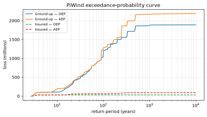
Exceedance-probability curve (EPT)

The EP table gives loss by return period. In ORD, EPType is 1=OEP, 2=OEP TVaR, 3=AEP, 4=AEP TVaR — where OEP is the largest single occurrence in a year, AEP is the year aggregate, and TVaR is the tail value-at-risk variant. EPCalc is the calculation basis (1=MeanDamage, 2=FullUncertainty, 3=PerSampleMean, 4=MeanSample); here we use Full Uncertainty (EPCalc 2). Below we plot the ground-up and insured OEP and AEP curves.

# ORD: EPType 1=OEP, 2=OEP TVaR, 3=AEP, 4=AEP TVaR;  EPCalc 2 = Full Uncertainty
ep_type_name = {1: "OEP", 3: "AEP"}

def load_ept(name):
    ept = pd.read_csv(OUT / name)
    return ept[ept["EPCalc"] == 2]                 # Full Uncertainty basis

gul_ept = load_ept("gul_S1_ept.csv")
il_ept = load_ept("il_S1_ept.csv")

fig, ax = plt.subplots(figsize=(7, 4))
for ept, perspective, style in [(gul_ept, "Ground-up", "-"), (il_ept, "Insured", "--")]:
    for etype in (1, 3):                            # OEP and AEP (skip their TVaR variants)
        g = ept[ept["EPType"] == etype].sort_values("ReturnPeriod")
        ax.plot(g["ReturnPeriod"], g["Loss"] / 1e6, style,
                label=f"{perspective} — {ep_type_name[etype]}")
ax.set_xscale("log")
ax.set_xlabel("return period (years)")
ax.set_ylabel("loss (millions)")
ax.set_title("PiWind exceedance-probability curve")
ax.legend(fontsize=8)
ax.grid(True, which="both", alpha=0.3)
fig.tight_layout()

Losses at key return periods

def loss_at(ept, etype, rp):
    g = ept[ept["EPType"] == etype].sort_values("ReturnPeriod")
    return np.interp(rp, g["ReturnPeriod"], g["Loss"])

targets = [10, 50, 100, 250]
summary = pd.DataFrame({
    "return_period": targets,
    "GUL_OEP_m": [loss_at(gul_ept, 1, t) / 1e6 for t in targets],   # EPType 1 = OEP
    "GUL_AEP_m": [loss_at(gul_ept, 3, t) / 1e6 for t in targets],   # EPType 3 = AEP
    "IL_AEP_m": [loss_at(il_ept, 3, t) / 1e6 for t in targets],
}).round(2)
summary

	return_period	GUL_OEP_m	GUL_AEP_m	IL_AEP_m
0	10	105.36	189.62	31.50
1	50	688.17	698.43	61.64
2	100	1199.88	1276.26	63.00
3	250	1554.84	1858.64	83.69

Where next

• The step-by-step companion (planned) decomposes the generated run_kernel.sh and shows each pytools tool and its intermediary data.

• The Oasis output formats and the modules that produce these tables are documented in the OasisLMF Outputs & results reference (linked from the aggregated Oasis docs).