How does the Simulation Methodology Work?
Basic Description – IBTrACS Hazard Data
This section provides a basic overview of how the simulation method works for IBTrACS hazard data. The simulation method can be broken down into a few distinct steps:
Step 1: Randomly select a number of different latitude-longitudes near the area of exposure. The user defines the number of locations to be randomly sampled (or number of simulations), in the simulation tab. Each random selection of a latitude-longitude is known as a “simulation”.
Step 2: Record the losses generated for each simulation in each year of the historical data. This step involves looking at the events in the hazard data and seeing which storms would have led to at least some damage by checking against the relevant intensity values set in the vulnerability tab. The losses for each event are then recorded by checking against your vulnerability curve. The years 1978-2021 are used for all basins here except the North Atlantic.
Step 3: Average the losses across all years in the historical data for each simulation. This gives us an average over all the simulation-years for each simulation in the history. Each observation of a particular year in the history for a given simulated location is known as a “simulation-year”.
Step 4: Apply a weighting between 0 and 1 to the average loss for each simulation. The weighting is based on how far away the simulated location is to the exposure (e.g., a simulation that was very close might get a weighting of 0.9, one that was far away might get a weighting of 0.1).
Step 5: Calculate the weighted average of the simulated average losses for each location calculated in the earlier steps. This is the “weighted simulation loss “.
Detailed Steps– IBTrACS Hazard Data
The next section goes through each of these steps in more detail and attempts to explain why each step is necessary to the approach.
Step 1: How and why do we sample different locations?
It may seem odd to randomly select locations that are different to your exposure, however this is an important step which prevents over-generalising from a limited history and is the founding principle of all catastrophe models. For example, if your exposure is within a very small area or is a single location, you could have been relatively lucky and not had any significant wind events despite some events having just missed that location in the recorded history. If we just used the history at the exposure point, we would assume there is zero risk when this is clearly not the case. It is important to capture some element of variability in our loss estimate.
When randomly sampling these points, what sort of limits should we apply on the types of locations we sample? Clearly it wouldn’t make sense to randomly select points anywhere in the world, as most of these would have very different weather patterns to our exposure and may not even be located in the same tropical cyclone basin.
The method used here only looks at locations that are within 5 times the average radius of maximum wind speed (also known as RMW) from a tropical cyclone. If you’re modelling an area, then the radius of this is added on to the RMW before multiplying (so zero for a single location). It is assumed in this model that the radius of maximum wind speed figure is 87.6km (see RMW in the glossary for more detail on why this figure was chosen). Written as a formula, the sampling area looks like this:
Distance from exposure to sample from = 5 x (Radius of Maximum Wind Speed of a Tropical Cyclone + Radius of Exposure)
As an example, if we were modelling a single location, we would look to sample any locations that are within 5 x (87.6 + 0) = 438km of the exposure. By contrast if we were looking to model an area with a radius of 50km, we would draw sample locations from points within 5 x (87.6 + 50) = 688km of the exposure.
Five times the RMW is selected as this gives a good spread of locations over the area with which to capture variability in nearby weather patterns. The area is also not so large that we are sampling from observations that are not at all relevant.
Random numbers are selected for each simulation for latitudes and longitudes that lie within the distance calculated above. These are then used in the subsequent calculations and represent our simulated locations.
The average radius of maximum wind speed is an important figure for another reason, as it is assumed if a location sits within this radius then the location is “hit” by the storm. This will be covered in more detail in Step 2.
Step 2: How do we calculate losses for each simulated location?
Now that we have our simulated locations, we need to check these against the storm tracks from the IBTrACS hazard data. We will then be able to work out which events would have historically led to losses. This is done by drawing a 87.6km radius around each sampled location/area and checking which storms in the history would have passed through this circle. If a storm’s track has taken it within 87.6km of the location/area, then it is assumed that this would have affected the location and potentially led to a loss. As mentioned in the section above, 87.6km represents the RMW and it is assumed if a location sits within this radius then the location is “hit” by the storm.
Maximum wind speeds for each event from the event set that are recorded as falling within this circle are checked against the vulnerability curve you have defined. This is then used to calculate the appropriate losses for each event. The losses generated by each storm are then recorded, giving us a complete history of all storms impacting each simulated location over the years.
Consider an example where we run two simulations using a cyclone hazard dataset that covers three years of data (2019-2021). The asset is a single location with a value of 100,000 USD and has one intensity value set at 178km/h at which 100% damage occurs. No damage occurs below this, so this is effectively a “stepped” vulnerability curve with just one step. The table below gives an idea of how the approach described above would work in practice, each row is an event in the hazard dataset that lies within a reasonable distance of the exposure.
Row Number |
Simulation Location Number |
Simulation-Year |
Max Wind Speed |
Distance from Location |
Loss (USD) |
|---|---|---|---|---|---|
1 |
1 |
2019 |
185km/h |
50km |
100,000 |
2 |
1 |
2019 |
200 km/h |
25km |
100,000 |
3 |
1 |
2020 |
220km/h |
90km |
0 |
4 |
1 |
2021 |
190km/h |
45km |
100,000 |
5 |
2 |
2019 |
185km/h |
40km |
100,000 |
6 |
2 |
2021 |
140km/h |
35km |
0 |
The event in row 3 doesn’t generate a loss despite exceeding the intensity value, as it lies further than 87.6km away from location 1 and is therefore deemed to have not affected it. The event in row 6 doesn’t generate a loss either as the wind speed is below 178km/h at which damage starts to occur.
Step 3: How do we get an expected loss for each simulation?
The individual event losses calculated in Step 2 are then added up by simulation-year, giving a picture of the total loss generated across each year of the history for each location. Losses are capped here at the total value of the asset. The reason this is done is that it is assumed if your asset is completely destroyed, it would take longer than the time between two (or more) storms to fully rebuild it. Once we have the losses for each year of this history, it is simply a case of averaging across these to get an average loss for each simulation. This is all we need to give us one view of the expected loss, the unweighted expected loss, which is a simple average of the loss from each simulation. Going back to the example in step 2, the table below shows how we get from the event data to a table of losses by simulation-year.
Row Number |
Simulation Location Number |
Simulation-Year |
Loss (USD) Before Capping at Asset Value |
Loss (USD) After Capping at Asset Value |
|---|---|---|---|---|
1 |
1 |
2019 |
200,000 |
100,000 |
2 |
1 |
2020 |
0 |
0 |
3 |
1 |
2021 |
100,000 |
100,000 |
4 |
2 |
2019 |
100,000 |
100,000 |
5 |
2 |
2020 |
0 |
0 |
6 |
2 |
2021 |
0 |
0 |
Notice that all years are listed here including those with no relevant events or losses. The impact of the capping at the asset value is shown in row 1. 100,000 is the asset value, and because this has already been breached by the first event in the year, the total loss is capped at this level and no further loss is generated by the second event. The next step is then to calculate a historical average loss across all years for each simulation.
Row Number |
Simulation Location Number |
Average Loss (USD) After Capping |
|---|---|---|
1 |
1 |
(100,000 + 0 + 100,000) / 3 = 66,666.7 |
2 |
2 |
(100,000 + 0 + 0) / 3 = 33,333.3 |
Unweighted Simulated Loss |
(33,333.33 + 66,666.7) / 2 = 50,000 |
For each simulation we are taking the total capped losses from the previous table and dividing these by the number of years of data to get an average. 2019-2021 is three years of data, hence the denominator of 3 above. This now gives us an average loss for each simulation, taking a straight average across the two simulations gives us the unweighted expected loss which is displayed in the bottom row. This assumes all simulations are given identical weight regardless of how far they are from the exposure. The unweighted expected loss forms one of the measures of expected loss in the Risk Explorer’s Loss Analysis tab.
Step 4: How do we weight each simulation?
To get a view that takes into account the distance of the simulations from the exposure, we need to work out how to appropriately weight each simulation. Simulations nearer the exposure are likely to be more relevant and generalisable than those further away. As such, closer locations should be given higher weights in the expected loss calculation.
Weightings for each simulation will all be between 0 and 1 and are generally expressed as percentages. The most intuitive way to think of the weightings themselves is in relative terms. A weighting of 0.8 can be thought of as 80% of the potential maximum weighting, but it can also be interpreted as being given 8 times more weight in the final calculation than an observation weighted at 10%.
There are a number of potential weighting methods that could be used here so it’s worth bearing in mind that there is a certain degree of judgement in this step. An exponential weighting function with a lambda parameter of 3.2 has been selected for calculating the weightings in this model based on scientific and actuarial expert judgement. The table below shows the different weightings for a single location at intervals of 50km away from the exposure to give some idea of how the weighting changes in practice:
Row Number |
Distance from Exposure |
Exponential Weighting |
|---|---|---|
1 |
0 |
100% |
2 |
50 |
69% |
3 |
100 |
48% |
4 |
150 |
33% |
5 |
200 |
23% |
There are a few desirable properties to this function and parameterisation that make the exponential a good choice. These are highlighted below:
The weighting decreases at a constant rate as we move away from the exposure. For a single location, the weighting decreases by 30% in relative terms for every 50km we move away from the exposure. E.g., the weighting at 100km from the exposure is 48%, which is 30% less than the 69% weighting for a location 200km from the exposure.
The weighting function drops off quickly initially but the absolute decrease in weights slows as we get further away. The reason for this is there is intuitively a bigger gap in usefulness of an observation 0km vs 50km away compared to an observation being 200km vs 250km away.
The weighting approaches zero as we get towards the edge of the potential sampling area.
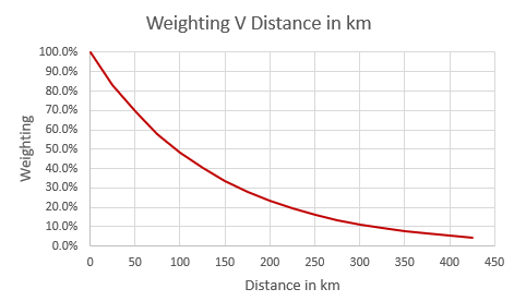
Exhibit demonstrating relationship between distance from exposure and weight for a single location.
Returning to our example in the earlier steps, these are the weightings that would be applied to each location:
Simulation Location Number |
Distance from Exposure |
Weighting |
|---|---|---|
1 |
125km |
40% |
2 |
200km |
23% |
A detailed understanding of how the exponential function is calculated is not necessary to use the tool, however if you are interested in learning more about this, you can consult the appendix section at the bottom of the page.
Step 5: How do we calculate the Simulated Weighted Loss?
The last step in getting our simulated weighted loss is calculating a weighted average. The losses for each simulation are scaled by their weightings and then divided by the sum of all weightings.
Returning to the earlier example, we can now calculate the simulated weighted loss:
Simulation Location Number |
Distance from Exposure |
Weighting |
Average Loss (USD) After Asset Value Capping |
Weighting x Average Loss |
|---|---|---|---|---|
1 |
125km |
40% |
66,666.7 |
0.4 x 66,666.7 = 26,733.35 |
2 |
200km |
23% |
33,333.3 |
0.23 x 33,333.3 = 7,733.33 |
Simulated Weighted Loss |
(26,733.35+ 7,733.33) / (4%+23%) = 54,449.73 |
In this case the expected weighted loss is 54,449.73. Note that this is higher than the expected unweighted loss of 50,000 which was calculated in step 3. The reason for this difference is that simulation 1 which had a higher average loss was given a higher weight in the calculation than simulation 2 which was lower. The reason for weighting location 1 higher is that it is closer to the exposure than location 2. In the unweighted calculation we implicitly assume all simulations have identical weighting so this generates a lower figure relative to the weighted loss.
The Weighting x Average Loss column doesn’t really have a practical interpretation but is shown to illustrate the different steps. The reason we need to divide by the sum of the weightings in the final calculation is to ensure we aren’t understating the total loss. If we just added together the Weighting x Loss column, this number wouldn’t account for the potential for a number of different weightings to emerge from the simulation process. This comes back again to the idea that the weightings themselves have more meaning when considered relative to one another, the sum of all weightings will differ each time a set of simulations is run so they need to be scaled accordingly. Note that if you are trying to recreate these figures, you may find small differences due to rounding.
Appendix: Step 4: How do we weight each simulation?
This section gives a brief demonstration of how we would go about calculating the exponential weightings described earlier. The calculation of these weightings relies on the mathematical constant “e” which is equal to 2.71828… .The formula for calculating the weighing is:
Weighting = e ^ ( (sim distance / max distance) x – (exponential parameter) )
Let’s assume we simulate a location that lies 150km from our exposure which is a single point. We also use the exponential parameter of 3.2 in the model. The weighting for this particular observation would be:
Weighting = e ^ ( (150/( 5 x 87.6)) x -3.2 )
Weighting = e^(-1.09589)
Weighting = 33.4%
This is the same weighting given in row 3 in the first table of step 4 (where it is rounded to one decimal place).
Basic Description – Stochastic Hazard Data
Step 1: Filter the events in the stochastic dataset that are relevant to your exposure. The stochastic dataset is made up of a large number of simulated years, each with their own specific events. The first step of the calculation excludes events that are too far away to impact your exposure area. Only events that occur within your exposure area are used in the subsequent calculations.
Step 2: Randomly select years from the dataset for each simulation. The selected years from the stochastic data and their corresponding events will then be used to calculate losses in later steps. Note that as the years in the stochastic data are selected at random, it is possible that certain years may repeat when a large number of simulations are run.
Step 3: Identify the events in each simulation that would lead to losses. This step looks at which events in your simulations would have led to losses based on values of the specified intensity measure in the vulnerability section. These losses are then summed up across each simulation-year and capped at your total asset value.
Step 4: Average across losses by simulation to give an overall expected loss. Each simulation should have a total loss associated with it calculated in step 3. This step averages across all of these simulation losses to give an overall expected loss.
Detailed Description – Stochastic Hazard Data
Step 1: How and why do we filter events relevant to the exposure? Unlike in the IBTrACS case where there are only a few tens of years of history to choose from, stochastic hazard data gives us thousands of simulated years to use. We therefore are able to focus on our exposure location/area exclusively and just look across the many years in the hazard data to generate variability in our modelling, rather than looking to different locations as we do with the IBTrACS historical sampling method. The hazard data for stochastic sets is split across four key files that sit behind the model:
areaperil_dict: This contains a list of all the lat-longs defining a particular “areaperil”. Areaperils are used to specify areas or locations that have the same intensity value in a given event
footprint: The footprint file lists all the events and the intensities for each areaperil.
intensity_bin_dict: This file contains the different values the intensity measure can take.
occurrence_lt: This file contains a list of the simulated years in the model and which events from the footprint file happened in those years
The footprint file is typically very large. Based on the values entered for your exposure, only the rows of the footprint file that relate to your exposure will be pulled in. A basic example of some of the key files is shown below to give an idea of the data that sits behind these stochastic sets. In this example there are 4 separate areas in our exposure all specified by a single latitude and longitude.
Areaperil |
Latitude |
Longitude |
|---|---|---|
1 |
0 |
0 |
2 |
1 |
0 |
3 |
0 |
1 |
4 |
0 |
1 |
The footprint file in this example contains two separate events that impact multiple different areas to varying degrees. For example event 101 impacts areaperils 1,2 and 4.
Event ID |
Areaperil ID |
Intensity bin ID |
|---|---|---|
100 |
1 |
4 |
100 |
2 |
5 |
101 |
1 |
3 |
101 |
4 |
3 |
101 |
2 |
4 |
The intensity bin table links the intensity bin id field in the footprint file to an actual intensity measure. In this example, wind speed is used. An intensity bin value of 3 corresponds to wind speeds of 120 km/h, a value of 4 to 130km/h and so on. To go back to the first row of the footprint file, we are saying that event 100 leads to wind speeds of 130km/h being recorded in area 1 and winds of 140km/h being recorded in area 2.
Intensity Bin ID |
Wind Speed |
|---|---|
1 |
100 km/h |
2 |
110km/h |
3 |
120 km/h |
4 |
130km/h |
5 |
140 km/h |
This file details which events occur in which simulated years. For year 3, both events 100 and 103 occur in the year. Note that some years have no events and consequently are not listed in the table (e.g. year 2)
Occurrence Number |
Event ID |
|---|---|
1 |
101 |
3 |
101 |
3 |
100 |
Step 2: Why are years randomly selected from the hazard data and how is this done? In many cases, the number of simulations you wish to model may be materially different than the number of simulated years in the occurrence_lt file. Randomly choosing years from the hazard data ensures that you have the correct number of simulations for your model run. This step is also where the different sub-files are joined together to create a full simulated event set, as they each store different types of information relating to intensity, location and frequency. This full event set for the exposure area can then be used to generate losses. Note that as the years in the stochastic data are selected at random, it is possible that certain years may repeat where a large number of simulations are being run. We run two simulations in the example, with occurrences 3 and 1 being chosen at random as can be seen in the table in step 3
Simulation Number |
Hazard Dataset Occurrence Number |
|---|---|
1 |
3 |
3 |
1 |
Step 3: How are losses generated? The next step is to generate losses for each individual event in the simulation data. This part of the process is very similar to the process for IBTrACS data. Given that the example in the IBTrACS section demonstrated how losses were generated for a step vulnerability curve, this example will look at a linear curve. Consider a linear vulnerability curve with 0% damage at 100 km/h and a 100% damage at 200km/h for an asset valued at USD 100,000. The table below shows the losses for the years selected in step 2:
Simulation Number |
Occurrence Number |
Event ID |
Intensity Measure (Wind Speed) |
Loss |
|---|---|---|---|---|
1 |
3 |
100 |
140km/h |
(140 – 100)/(200 – 100) = 40% damage x 100,000 = USD 40,000 |
1 |
3 |
101 |
130km/h |
(130 – 100)/(200 – 100) = 30% damage x 100,000 = USD 30,000 |
2 |
1 |
101 |
130km/h |
(130 – 100)/(200 – 100) = 30% damage x 100,000 = USD 30,000 |
The linear losses are calculated by looking at how far the intensity measure lies between the specified intensity measure values. As 140 km/h is 40% of the way between 100km/h and 200 km/h, this means a 40% loss is sustained for this wind speed. Now we just add all the losses across each simulation number to get losses by simulation.
Simulation Number |
Occurrence Number |
Total Loss |
|---|---|---|
1 |
3 |
USD 40,000 |
2 |
1 |
USD 60,000 |
Step 4: How is the expected simulation loss generated? The final step here is to average across all our simulations to give an expected annual simulation loss. The losses for all years are summed together and divided by the number of simulations to give the average as below.
Simulation Number |
Occurrence Number |
Total Loss |
|---|---|---|
1 |
3 |
USD 40,000 |
2 |
1 |
USD 60,000 |
Simulated Loss |
(40,000+60,000)/2 = USD 50,000 |
Note there is only one simulation method here, this is because the concept of weightings is not used as all simulations relate to the exposure area. There is also no historical data available to give the historic simulation, although this could be calculated in principle with the right data available.