Analyse ORD results: from an ELT to an EP curve
Run this tutorial yourself
This page is a Jupyter notebook, executed when the docs are built. Download analyse-ord-results.ipynb
Set up an environment and open it in Jupyter:
python -m venv venv && source venv/bin/activate
pip install oasislmf jupyterlab matplotlib
jupyter lab analyse-ord-results.ipynb
The example data ships in the OasisLMF repository (under docs/source/tutorials/); tutorials that run a model need that model’s data and the loss engine — follow the prerequisites described on this page.
The Open Results Data (ORD) standard defines the result tables Oasis produces —
event loss tables (ELT), period loss tables (PLT), and exceedance-probability
tables (EPT). This notebook builds a small event loss table, simulates a
year loss table, and derives an EP curve (OEP and AEP) — the same chain the
pytools output modules (elt, plt, lec) implement.
Note
Executable notebook — run at build time. It uses only synthetic data so it is fully
self-contained. For the Oasis output implementation see Outputs & results;
the ORD standard itself is single-sourced in the ODS_OpenResultsData repository.
import numpy as np
import pandas as pd
import matplotlib.pyplot as plt

rng = np.random.default_rng(42)  # fixed seed → reproducible build
Matplotlib is building the font cache; this may take a moment.
An event loss table (ELT)
Each event has an occurrence rate (events per year) and a loss distribution (mean and standard deviation). This is the analytical ELT — the SELT/MELT family in ORD terms.
n_events = 40
elt = pd.DataFrame({
    "event_id": np.arange(1, n_events + 1),
    "rate": rng.uniform(0.005, 0.15, n_events),          # annual occurrence rate
    "mean_loss": rng.lognormal(mean=15.0, sigma=1.0, size=n_events),
})
elt["sd_loss"] = elt["mean_loss"] * rng.uniform(0.3, 0.8, n_events)
elt.head()
| event_id | rate | mean_loss | sd_loss | |
|---|---|---|---|---|
| 0 | 1 | 0.117224 | 6.873982e+06 | 4.859976e+06 |
| 1 | 2 | 0.068637 | 5.627379e+06 | 2.158023e+06 |
| 2 | 3 | 0.129497 | 1.680312e+06 | 5.231754e+05 |
| 3 | 4 | 0.106118 | 4.123287e+06 | 1.422633e+06 |
| 4 | 5 | 0.018656 | 3.673612e+06 | 2.428917e+06 |
Simulate a year loss table (YLT)
Sample many years; in each year an event occurs with probability equal to its rate, and its loss is drawn from a lognormal matching the ELT mean/sd.
n_years = 20_000

# lognormal parameters from each event's mean/sd
cv = elt["sd_loss"].to_numpy() / elt["mean_loss"].to_numpy()
sigma = np.sqrt(np.log(1 + cv**2))
mu = np.log(elt["mean_loss"].to_numpy()) - sigma**2 / 2

occurs = rng.random((n_years, n_events)) < elt["rate"].to_numpy()      # year × event
sampled = np.exp(rng.normal(mu, sigma, size=(n_years, n_events)))
year_event_loss = np.where(occurs, sampled, 0.0)

oep_year = year_event_loss.max(axis=1)   # largest single occurrence per year
aep_year = year_event_loss.sum(axis=1)   # aggregate loss per year
print(f"{n_years:,} simulated years; "
      f"mean annual loss = {aep_year.mean():,.0f}")
20,000 simulated years; mean annual loss = 12,589,217
Derive the EP curve (EPT)
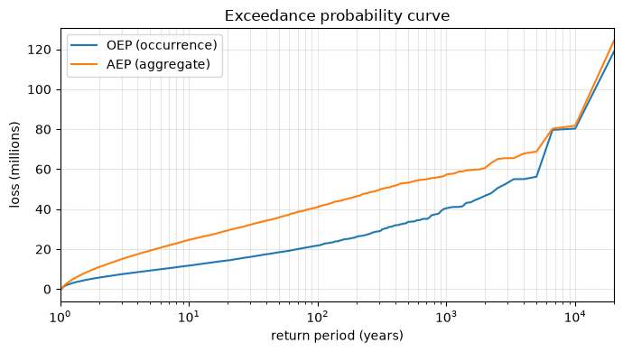
The exceedance-probability curve ranks the per-year losses; the return period is the reciprocal of the exceedance probability. OEP uses the per-year maximum occurrence; AEP uses the per-year aggregate.
def ep_curve(period_losses):
    """Return (return_period, loss) sorted from rare (high RP) to frequent."""
    loss = np.sort(period_losses)[::-1]              # descending
    ep = np.arange(1, len(loss) + 1) / (len(loss) + 1)
    return 1.0 / ep, loss                            # return period, loss

rp_oep, loss_oep = ep_curve(oep_year)
rp_aep, loss_aep = ep_curve(aep_year)

fig, ax = plt.subplots(figsize=(7, 4))
ax.plot(rp_oep, loss_oep / 1e6, label="OEP (occurrence)")
ax.plot(rp_aep, loss_aep / 1e6, label="AEP (aggregate)")
ax.set_xscale("log")
ax.set_xlim(1, n_years)
ax.set_xlabel("return period (years)")
ax.set_ylabel("loss (millions)")
ax.set_title("Exceedance probability curve")
ax.legend()
ax.grid(True, which="both", alpha=0.3)
fig.tight_layout()
Losses at key return periods
The numbers a report cares about — the loss at standard return periods, interpolated from the EP curve:
def loss_at(rp, loss, target):
    # ep_curve returns descending; reverse to ascending return period for interp
    return np.interp(target, rp[::-1], loss[::-1])

targets = [10, 50, 100, 250]
summary = pd.DataFrame({
    "return_period": targets,
    "OEP_loss_m": [loss_at(rp_oep, loss_oep, t) / 1e6 for t in targets],
    "AEP_loss_m": [loss_at(rp_aep, loss_aep, t) / 1e6 for t in targets],
}).round(1)
summary
| return_period | OEP_loss_m | AEP_loss_m | |
|---|---|---|---|
| 0 | 10 | 11.7 | 24.6 |
| 1 | 50 | 18.4 | 35.8 |
| 2 | 100 | 21.8 | 41.0 |
| 3 | 250 | 27.5 | 48.3 |
Where next
Outputs & results — the Oasis output formats and the
elt/lec/pltmodules that generate these tables.ORD output components — how the kernel emits ORD outputs.
Sampling Methodology — how sampled losses feed these curves.