Explore Oasis model data
Run this tutorial yourself
This page is a Jupyter notebook, executed when the docs are built. Download explore-model-data.ipynb
Set up an environment and open it in Jupyter:
python -m venv venv && source venv/bin/activate
pip install oasislmf jupyterlab matplotlib
jupyter lab explore-model-data.ipynb
The example data ships in the OasisLMF repository (under docs/source/tutorials/); tutorials that run a model need that model’s data and the loss engine — follow the prerequisites described on this page.
A hands-on look at the data that drives a ground-up loss calculation — the footprint, vulnerability, and damage bin dictionary (model static data) plus the items and coverages (the exposure). This notebook loads a small example model shipped with the docs and inspects each file with pandas.
Note
This page is an executable notebook — every cell below is run when the docs are built, so the outputs are always produced against the current code and data. See Explanation for the concepts and Reference for the file-format reference.
from pathlib import Path
import pandas as pd
import matplotlib.pyplot as plt

# Resolve the example-data directory regardless of the notebook's execution cwd.
_candidates = [
    Path("data/example_model"),
    Path("tutorials/data/example_model"),
    Path("docs/source/tutorials/data/example_model"),
]
DATA = next((c for c in _candidates if c.exists()), None)
assert DATA is not None, "example_model data directory not found"
DATA
PosixPath('data/example_model')
Damage bins
Damage is discretised into bins. The damage bin dictionary defines the interval
each bin covers (bin_from–bin_to) — losses are sampled as bin indices and later
mapped back to a mean damage ratio.
damage_bins = pd.read_csv(DATA / "damage_bin_dict.csv")
damage_bins.head()
| bin_index | bin_from | bin_to | interpolation | damage_type | |
|---|---|---|---|---|---|
| 0 | 1 | 0.0 | 0.0 | 0.00 | 0 |
| 1 | 2 | 0.0 | 0.1 | 0.05 | 0 |
| 2 | 3 | 0.1 | 0.2 | 0.15 | 0 |
| 3 | 4 | 0.2 | 0.3 | 0.25 | 0 |
| 4 | 5 | 0.3 | 0.4 | 0.35 | 0 |
Footprint
The footprint gives, for each event, a probability distribution over hazard intensity bins at each area-peril (grid cell). It is the hazard side of the calculation.
footprint = pd.read_csv(DATA / "footprint.csv")
print(f"{footprint['event_id'].nunique()} events, "
      f"{footprint['areaperil_id'].nunique()} area-perils")
footprint.head()
4 events, 110 area-perils
| event_id | areaperil_id | intensity_bin_id | probability | |
|---|---|---|---|---|
| 0 | 1 | 3 | 1 | 1.0 |
| 1 | 1 | 4 | 1 | 0.2 |
| 2 | 1 | 4 | 2 | 0.6 |
| 3 | 1 | 4 | 3 | 0.2 |
| 4 | 1 | 5 | 1 | 0.2 |
Vulnerability
The vulnerability functions give, for each vulnerability id, the probability of each damage bin conditional on the hazard intensity bin — i.e. how damageable a coverage is at a given intensity.
vulnerability = pd.read_csv(DATA / "vulnerability.csv")
vulnerability.head()
| vulnerability_id | intensity_bin_id | damage_bin_id | probability | |
|---|---|---|---|---|
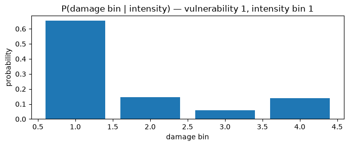
| 0 | 1 | 1 | 1 | 0.654 |
| 1 | 1 | 1 | 2 | 0.146 |
| 2 | 1 | 1 | 3 | 0.060 |
| 3 | 1 | 1 | 4 | 0.140 |
| 4 | 1 | 2 | 1 | 0.654 |
Below is the conditional damage distribution for one vulnerability function at one hazard intensity — the building block the Monte-Carlo engine samples from:
vid = int(vulnerability["vulnerability_id"].iloc[0])
iid = int(vulnerability.loc[vulnerability.vulnerability_id == vid, "intensity_bin_id"].iloc[0])
sub = vulnerability[(vulnerability.vulnerability_id == vid)
                    & (vulnerability.intensity_bin_id == iid)]

fig, ax = plt.subplots(figsize=(7, 3))
ax.bar(sub["damage_bin_id"], sub["probability"])
ax.set_xlabel("damage bin")
ax.set_ylabel("probability")
ax.set_title(f"P(damage bin | intensity) — vulnerability {vid}, intensity bin {iid}")
fig.tight_layout()
Exposure: items and coverages
Coverages hold the insured values (TIV); items link each coverage to an area-peril and a vulnerability function (the join between exposure and model data).
items = pd.read_csv(DATA / "items.csv")
coverages = pd.read_csv(DATA / "coverages.csv")
exposure = items.merge(coverages, on="coverage_id")
print(f"{len(items)} items across {len(coverages)} coverages; "
      f"total TIV = {coverages['tiv'].sum():,.0f}")
exposure.head()
10 items across 10 coverages; total TIV = 3,400,000
| item_id | coverage_id | areaperil_id | vulnerability_id | group_id | tiv | |
|---|---|---|---|---|---|---|
| 0 | 1 | 1 | 154 | 8 | 833720067 | 220000.0 |
| 1 | 2 | 1 | 54 | 2 | 833720067 | 220000.0 |
| 2 | 3 | 2 | 154 | 8 | 956003481 | 790000.0 |
| 3 | 4 | 2 | 54 | 2 | 956003481 | 790000.0 |
| 4 | 5 | 3 | 154 | 8 | 335506702 | 160000.0 |
Where next
Modelling methodology and Sampling Methodology — how these inputs become sampled losses.
Compute ground-up losses with gulmc — run the gulmc engine on data like this.
Oasis Model Data Formats — the full file-format reference.