Disaggregation
On this page
Introduction
Oasis is a detailed loss modelling platform, meaning that it is designed for modelling individual buildings with known locations and vulnerability attributes. However, exposure data can be aggregated, low resolution or missing key attributes. This is particularly true in the developing world - a key focus of the Oasis model library.
Uncertainty about the exposures is not always captured in loss output. In the modelling process we try to find a best match of an exposure’s location to the model’s hazard grid (areaperil_id) and a vulnerability function (vulnerability_id) which together determine the effective damage distribution per event in the analysis. But where full exposure detail is missing, other choices of areaperil_id and vulnerability_id might be valid and produce a different distribution and therefore different losses.
Oasis has implemented a range of options to support different ways of handling of uncertainty in the exposure inputs to improve the quality of risk modelling across all models. This was completed in 2023 following consultation of a technical steering subgroup representing model vendors, and model development teams within reinsurance brokers and risk carrier organisations.
Our toy model PiWind Postcode demonstrates the disaggregation features of Oasis. This model is availible to use from here.
Disaggregation features by version
There are a few options in Oasis to handle disaggregation, and more features have been added in the more recent oasislmf package versions.
These can be summarized as follows;
- 1.15 and later
Pre-analysis hooks for model-specific disaggregation
Aggregate footprints to represent exposure location uncertainty
- 1.27 and later
On-the-fly blended vulnerability for unknown risk attributes
- 1.28 and later
Number of buildings disaggregation
Financial terms disaggregation
Available in OasisLMF 1.15
Pre-analysis hooks
For versions of OasisLMF before 1.28, aggregate exposure data must be converted into detailed data, one building per row in the location file, before being imported into the platform for analysis. This can be done outside of the system or the model developer, as part of the Oasis model assets, may provide a pre-analysis routine to generate a modified OED location file from an input OED location file which splits aggregate risk records into detailed risk records.
The purpose of pre-analysis routines are to provide flexibility to manipulate the OED input files before the model is run, for augmentation as required by the model.
Some examples of the procedures that might be applied in a pre-analysis hook are as follows;
spatial disaggregation - where total insured value of an exposure location known at admin zone level is distributed to the co-ordinates of a high resolution grid.
risk attribute augmentation - where missing risk attributes or general occupancy/construction codes are replaced with more specific risk attributes based on a built environment dataset
number of risks disaggregation - where a single row in the exposure input represents multiple buildings (‘aggregate’ exposure data) is split out into one building per row
combinations of the above
Pre-analysis hooks consist of modeller-provided source code and sometimes reference datasets containing built environment information. The hooks can be invoked at the very start of the model run workflow to generate a modified set of OED input files before the Oasis kernel exposure files are prepared.
A very simple pre-analysis ‘hook’ for the PiWind model which demonstrates the mechanism can be found here.
See the pre-analysis hooks section for more information about how to use them.
Aggregate footprints to represent exposure location uncertainty
If the geographical location of an exposure known at a lower resolution than the model’s hazard footprint (which typically requires street address or latitude-longitude precision) then whether it can be modelled or not depends on the model. Each Oasis model will specify a list of geographical fields required for modelling. This could be just the latitude-longitude point, or it could be latitude-longitude point and/or postal code, etc, because hazard data is normally provided at a very detailed level, depending on the peril in question.
Geocoding may be performed to find the coordinates for the exposure as a pre-import step, but this is unlikely to improve the ability of the model to produce reliable risk results. This is because geocoding will typically return the latitude-longitude centroid of the administrative zone for the exposure. Any exposure with this address level will be matched with the closest hazard cell in the model to the centroid point and the uncertainty over the exact location of the exposures within the administrative zone, along with the chance of it experiencing a range of hazard intensities, is ignored.
A spatial disaggregration pre-analysis hook as described above is a good way of distributing exposure value to model cells to capture the range of hazard intensities the exposure might experience. The disadvantage is that for very low resolution admin zones, this can result in an explosion of the number of location records in the disaggregated location file, which may be too big or very slow to run an analysis on.
An alternative way to handle location uncertainty is for the modeller to build a set of hazard footprints at the same resolution that the geographical location is known.
As an example, taking a hypothetical area grid which contains 9 smaller grid cells. Each small grid cell contains a hazard intensity value, represented here by bin index 1, 2 or 3. A hazard intensity distribution can be created for the large area grid by binning the hazard values of the 9 grid cells.
Uniform binning of intensity to aggregate cell level
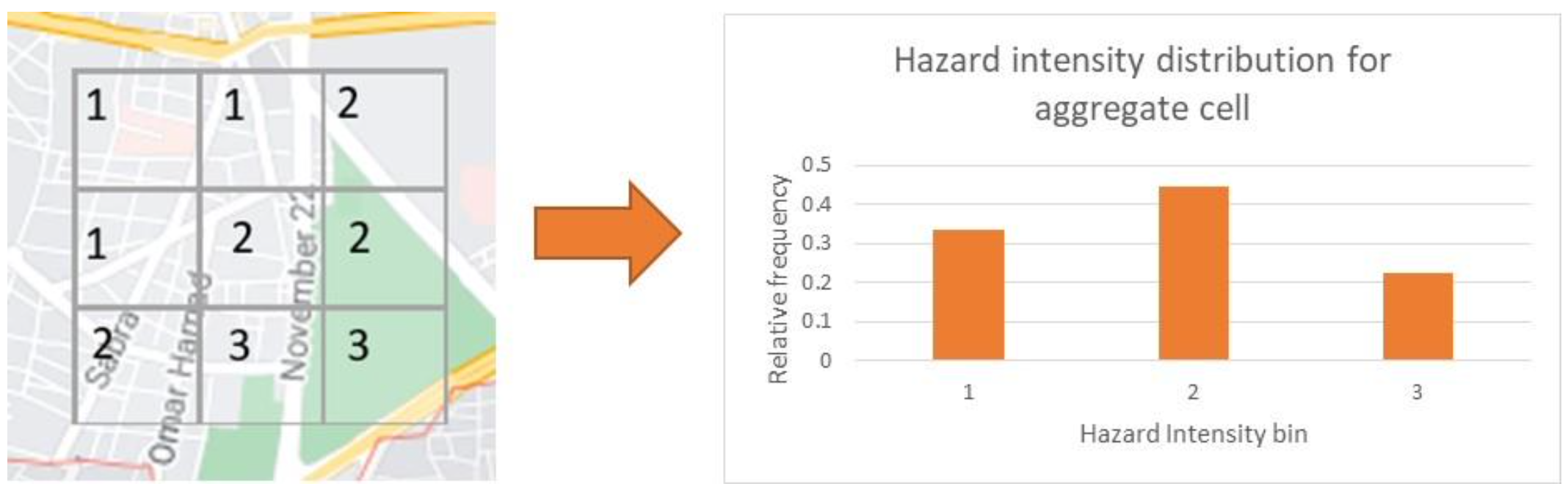
This method could be performed for any definition of area, such as administrative zone, although irregular boundaries make it more complicated.
If information about the built environment is known, a more sophisticated approach is to weight the values according to where the buildings are concentrated.
Weighted binning of intensity to aggregate cell level
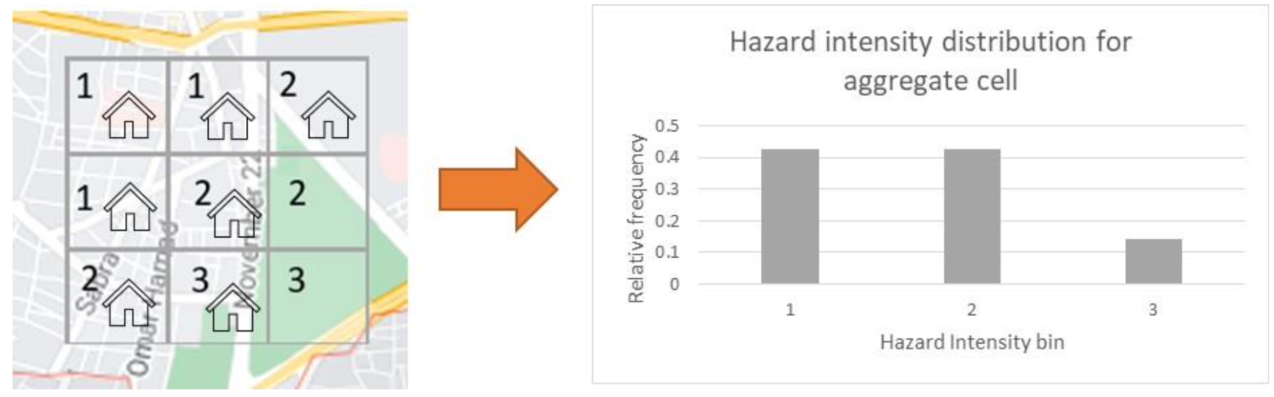
The weighting can further be based on some measure of building density within each small grid. These binned distributions can be included in the model hazard footprint as ‘aggregate’ footprints against a different range of areaperil_ids and exposures can be matched to these footprints as appropriate.
The relative frequencies are interpreted as probabilities of an exposure experiencing different levels of hazard intensity for an event, which proxies the uncertainty of the precise location. These probabilities can be represented in the footprint by intensity bin, for each event and areaperil.
Both fine-grid hazard intensity footprints and aggregate footprints for the low resolution admin zones can be stored in the same footprint file. This means that an exposure location can be matched to the fine-grid footprint when its lat-lon is known, or to the aggregate footprint for the admin zone otherwise. Multiple levels of admin zones can be stored in the footprint if required.
Available in OasisLMF 1.27
On-the-fly blended vulnerability for unknown risk attributes
Vulnerability attributes that determine the damage response to a given level of hazard intensity in a vulnerability module are typically peril, coverage type, occupancy and/or construction type. There is a long list of other data fields that are used as modifiers to the damage response for a general type of building, but very often in exposure data the more detailed information is missing, and modellers have to support the minimum set of fields.
To handle this, and as an alternative to writing a pre-analysis hook to augment input exposure data for missing risk attributes, modellers will often provide vulnerability functions for general residential or commercial lines of business, etc. These base functions are independent of location and assume a static mixture of vulnerability functions for the supported types (e.g. detached house, 2 storeys, 1960’s build and all the various combinations), often with wider overall uncertainty as a result of being a blend of many different distributions.
If information about the built environment is known, then based on where the location is, the modeller can instead blend vulnerability functions based on the known mixture of building types in the local area. This can greatly improve the modelling of vulnerability compared with the general functions and reduce the modelled uncertainty associated with unknown attributes.
Vulnerability modules can have quite small file sizes when the functions are independent of location. However, adding area-based vulnerability curves to an Oasis vulnerability module (e.g. one for every postcode) can make the file size infeasbily large. This is a bigger issue for the vulnerability module than it is to append aggregate footprints to the detailed footprint, where the detailed footprints are already very big and the increase in file size is relatively small.
Oasis has implemented on-the-fly blending of vulnerability damage distributions for missing risk attributes, to remove the necessity to pre-calculate and store area-based vulnerability curves. This requires the model provider to prepare two extra model files;
aggregate_vulnerability - this defines a new range of vulnerability ids identifying different mixtures of unknown attributes ‘aggregate_vulnerability_id’ and maps them to the vulnerability_ids for known risk attributes. This is a small file as it is area-independent.
weights - for each areaperil in the model, this defines the list of vulnerability_ids for known risk attributes (i.e. not aggregate_vulnerability_ids) that are present. A third ‘count’ field stores any measure of exposure concentration such as population, sum insured or other economic measure. It is used to derive relative weights for weighting the damage probability distributions contained within the vulnerability file for the vulnerability_ids present for each areaperil_id. This can be a very large file.
The model provider must also include the set of aggregate vulnerability ids in the vulnerability dictionary along with their risk attributes (which will be a mixture of known and unknown attributes) so that exposures may be matched to them during the keys lookup process.
Wherever exposures are matched with an aggregate_vulnerability_id in the keys lookup process, a dynamic weighting of the damage distributions for known attributes in the kernel is invoked during the model execution. The weighting is based on the ‘count’ data provided in the weights file.
The model files can be in csv or binary format. The data structures with example data are as follows;
aggregate_vulnerability:
aggregate_vulnerability_id |
vulnerability_id |
|---|---|
100001 |
101 |
100001 |
102 |
100001 |
103 |
100002 |
104 |
100002 |
105 |
100002 |
106 |
weights;
areaperil_id |
vulnerability_id |
count |
|---|---|---|
1 |
101 |
300 |
1 |
102 |
200 |
2 |
101 |
100 |
2 |
103 |
400 |
1001 |
101 |
400 |
1001 |
102 |
600 |
1001 |
103 |
300 |
The areaperil_id column can include areaperil_ids for ‘aggregate’ footprints if provided in the hazard footprint.
It is necessary to use the gulmc calculation module to use this feature. For more details please see Pytools gulmc
Available in OasisLMF 1.28
Number of buildings disaggregation
Oasis has implemented a default dissaggregation rule to split each exposure location into a number of ‘subrisks’ based on the NumberOfBuildings field in the OED location file for the purposes of ground up loss modelling. This is as an alternative to both manual disaggregation by the user pre-import and having to rely on the modeller to provide a pre-analysis disaggregation (which they may not do). This logic will apply when running against any model in the Oasis platform.
The user location file is not disaggregated itself, as it would be using a pre-analysis hook, but instead the disaggregation is performed as a final step in the exposure file preparation stage. This is a more space-efficient way of expanding the number of risks to be modelled.
The total insured value for each coverage is split equally by the value in the NumberOfBuildings field.
Expanded items file
Multiple records will be created in the kernel inputs files for each disaggregated risk. The reference information is kept in the gul_summary_map file as normal.
The following example shows the disaggregated kernel files for two aggregate locations represents 5 individual risks.
OED location:
Port Number |
Acc Number |
Loc Number |
NumberOfBuildings |
BuildingTIV |
|---|---|---|---|---|
3 |
3 |
Loc1 |
2 |
500,000 |
3 |
3 |
Loc2 |
3 |
600,000 |
items:
item_id |
coverage_id |
areaperil_id |
vulnerability_id |
damage_group_id |
|---|---|---|---|---|
1 |
1 |
100001 |
101 |
1 |
2 |
2 |
100001 |
101 |
1 |
3 |
3 |
100002 |
101 |
2 |
4 |
4 |
100002 |
101 |
2 |
5 |
5 |
100002 |
101 |
2 |
gul_summary_map:
loc_id |
PortNumber |
AccNumber |
LocNumber |
loc_idx |
peril_id |
coverage_type_id |
tiv |
coverage_id |
item_id |
layer_id |
agg_id |
|---|---|---|---|---|---|---|---|---|---|---|---|
1 |
3 |
3 |
Loc1 |
0 |
WTC |
1 |
250,000 |
1 |
1 |
1 |
1 |
1 |
3 |
3 |
Loc1 |
0 |
WTC |
1 |
250,000 |
2 |
2 |
1 |
2 |
2 |
3 |
3 |
Loc2 |
1 |
WTC |
1 |
200,000 |
3 |
3 |
1 |
3 |
2 |
3 |
3 |
Loc2 |
1 |
WTC |
1 |
200,000 |
4 |
4 |
1 |
4 |
2 |
3 |
3 |
Loc2 |
1 |
WTC |
1 |
200,000 |
5 |
5 |
1 |
5 |
Financial terms disaggregation
When the number of buildings in the OED input location file is greater than 1, there are two main situations which distinguish how location level financial terms should apply;
The row represents a single site of multiple buildings, such as a campus or caravan park.
The row represents aggregate exposure, i.e. multiple separate risks/sites of a similar risk type and geographical location.
Although the ground up loss modelling treatment is the same for both cases, it is necessary to distinguish between the two due to:
The classification of a multi-building site as a single risk from the perspective of the insurer and the application of policy terms and conditions at the site level rather than the individual building level.
The closer proximity of the individual buildings, leading to potentially stronger correlation in hazard and damage
The IsAggregate field in the OED location file can be used to distinguish between these two uses of the NumberOfBuildings field
IsAggregate = 0 (default) means that the row represents a single site with multiple buildings.
IsAggregate = 1 means that the row represents aggregate data.
In both cases ground up losses will be modelled for each individual building. However, for campus sites the insurance policy terms will generally be applicable at the site level, so that ground up losses should be aggregated back up to the site level before policy ‘location’ level deductibles and limits are applied (all the financial fields that begin with ‘Loc’).
For aggregate data, location financial terms are treated the same as TIV, they are split and applied to each disaggregated risk.
Here are the six possible combinations of NumberOfBuildings and IsAggregate, and how each is interpreted in Oasis;
Case |
NumberOfBuildings |
IsAggregate |
Description |
|---|---|---|---|
1 |
1 |
0 |
Default case. Single risk single building |
2 |
n>1 |
1 |
Aggregate data with n risks |
3 |
n>1 |
0 |
Single risk site/campus with n buildings |
4 |
0 |
1 |
Aggregate data with unknown number of risks |
5 |
0 |
0 |
Assume default case. Single risk, single building |
6 |
1 |
1 |
Assume default case. Single risk, single building |
The disaggregation and financial terms treatment for each case are as follows;
Case |
Disaggregation treatment |
Financial terms treatment |
|---|---|---|
1 |
No disaggregation |
Location terms apply per risk |
2 |
Disaggregate to n subrisks |
Location terms apply per subrisk |
3 |
Disaggregate to n subrisks |
Location terms apply per risk |
4 |
No disaggregation |
Location terms apply per risk |
5 |
As for case 1 |
As for case 1 |
6 |
As for case 1 |
As for case 1 |
Monetary financial deductibles and limits are split equally by the number of buildings for case 2 to be applied to each subrisk in the financial calculations. Percentage deductibles and limits are unchanged and apply to each subrisk.
The calculation logic is driven directly from the user input location data on a record by record basis, depending on which of the six cases above it matches. There is no command switch to stop the number of risks disaggregation from occurring.
It is necessary to use the gulmc calculation module to use this feature. For more details please see Pytools gulmc
Correlation of disaggregated risks
There is also a difference between the two IsAggregate cases in how disaggregated risks are grouped for the purposes of correlating hazard and damage in the ground up loss calculation.
The model provider can control this through the model settings json.
In case it is not specified, the default setting in Oasis is to fully correlate the subrisks for campus sites in case 3 (same correlation group id is assigned) and to make the subrisks for aggregate data independent in case 2 (different correlation group_id per subrisk).
For more details on model provider controls for correlation, please see Correlation