Sampling Methodology
On this page
Introduction
This section explains the full ground up loss calculation, which consists of two main stages;
calculation of probability distributions
the sampling method
This section cover the inputs to the ground up loss calculation and how they control the random numbers that are drawn, the seeding of random numbers, the algorithms used to draw random numbers and the method of generating partially correlated random numbers more recent releases of Oasis.
Sampling features by version
More features have been added in the more recent oasislmf package versions.
These can be summarized as follows;
- 1.27
Latin Hypercube sampling
Partially correlated random numbers for damage
Full Monte Carlo Sampling
Partially correlated random numbers for hazard intensity
Effective damageability method
Effective damageability is the name of the method used for the construction of probability distributions.
The model input files to this stage of the calculation are;
footprint
vulnerability
Hazard intensity uncertainty is represented in the footprint data, and damage uncertainty given the hazard intensity is represented in the vulnerability data. Both types of uncertainty are represented as discrete probability distributions.
Effective damage is calculated during an analysis by combining (‘convolving’) the hazard intensity distribution with the conditional damage distribution.
In the general case, the calculated effective damage distribution represents both uncertainty in the hazard intensity and in the level of damage given the intensity.
However it is common in models to have no hazard uncertainty distribution in the footprint. This is when each areaperil (representing a geographical area/cell) in the footprint is assigned a single hazard intensity bin with probability set to 1. In this case, the effective damage distribution is still generated but it is the same as the conditional damage probability distribution in the vulnerability file for a single intensity bin.
Under the effective damageability method, it is always the effective damage distribution that is sampled, but the sources of uncertainty that are represented may be just damage, or may be a combination of hazard intensity uncertainty and damage uncertainty, depending on the model files.
Monte Carlo sampling
Monte Carlo methods are a broad class of computational algorithms that rely on repeated random sampling to obtain numerical results.
The Oasis kernel performs a Monte Carlo sampling of ground up loss from effective damage probability distributions by drawing random numbers.
The probability distribution is provided by the effective damageability calculation described above, and the damage intervals are provided by a third model input file, the damage bin dictionary.
Exposure inputs
The exposure data input files control all aspects of how ground up losses are sampled. The inputs are two related files;
items
coverages
Items are the smallest calculation unit in Oasis, and they represent the loss to an individual coverage of a single physical risk from a particular peril. The coverage file lists the exposure coverages (for example the building coverage of an individual site) with their total insured values.
The attributes of items are;
item_id - the unique identifier of the item
coverage_id - identifier of the exposure coverage that an item is associated with (links to the coverages file)
areaperil_id - identifier which determines what event footprints will impact the exposure and with what hazard intensity
vulnerability_id - identifier which determines what the damage severity will be given the hazard intensity
group_id - identifier that generates a set of random numbers that will be used to sample loss
The attributes of coverages are;
coverage_id - the unique identifier of the exposure coverage
tiv - the total insured value of the coverage
For each item, the values of areaperil_id and vulnerability_id determine the inputs to the calculation of the effective damage distribution for each event, the group_id determines which set of random numbers will be used to sample damage, and the coverage_id determines what tiv the damage factor will be multiplied by to generate a loss sample.
See correlation.rst for more information about how group_ids are generated.
Random number seeding
A random number set is seeded from the input keys ‘event_id’ and ‘group_id’. This means that for each unique set of values of ‘event_id’ and ‘group_id’, an independent set of random numbers is drawn. The size of the random number set is determined by the number of samples specified in the analysis settings.
Seeded random number sets are repeatable. This means that for the same value of ‘event_id’ and ‘group_id’, the set of random numbers generated will always be the same.
Whereever items are assigned the same group_id, the same set of random numbers will be used to sample ground up losses. The damage samples are fully correlated for these items, whereas they are uncorrelated to all items with different assigned group_ids.
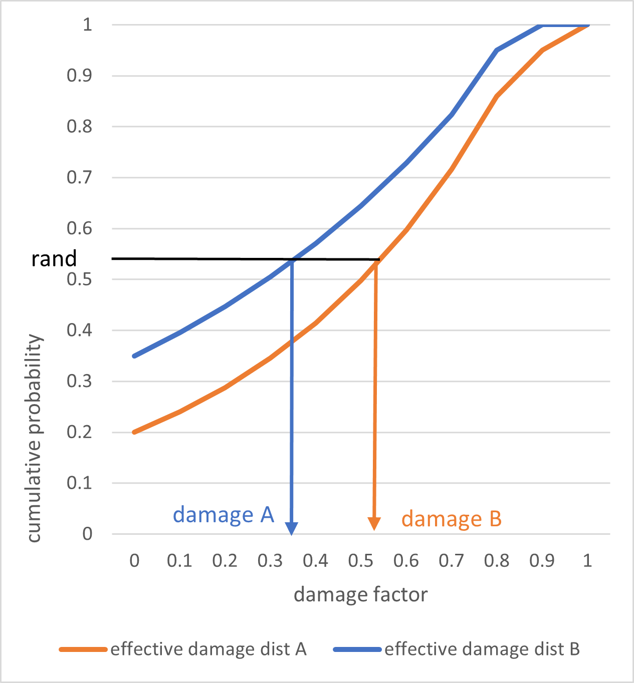
Note that just because the random numbers used to sample from two item’s damage distributions are the same does not mean the sampled damage factors will be the same. The damage factor will also depend on the cumulative distribution function, which will vary across items.
However, damage samples will have ‘rank’ correlation, meaning that the largest damage factors for two fully correlated items across the sample set will occur together, and the second largest damage factors will occur together, and so on.
Full correlation sampling across two different effective damage cdfs
Inverse transform sampling
Inverse transform sampling is a basic method for psuedo-random number sampling, i.e. for generating sample numbers at random from any probability distribution given its cumulative distribution function.
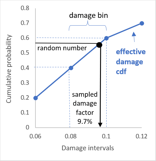
In Oasis, all probability distributions are discrete. The cumulative probability is calculated for each damage interval threshold and the random number (a value between 0 and 1) is matched to a damage bin when its value is between the cumulative probability lower and upper threshold for the bin. Linear interpolation is performed between the lower and upper cumulative probability thresholds to calculate a damage factor between 0 and 1.
Inverse transform method for a discrete cumulative distribution function
Each damage factor is multiplied by the total insured value of the exposed asset to produce a ground up loss sample. This is performed at the individual building coverage level, for each modelled peril, for every event in the model. This is repeated for the number of samples specified for the analysis.