Financial Module
On this page
Introduction
The Oasis framework supports a wide range of financial calculations. Outputs can be generated for three perspectives:
Ground-up: the underlying cost of loss.
Insured loss: the loss ceded to the direct insurance contracts.
Net loss: the insured loss net of reinsurance recoveries.
Exposure is uploaded in the OED exposure format. See here for full details. A full list of OED financial terms suppported by the Financial Module can be found in OED_financial_terms_supported.xlsx.
Supported OED terms
The Financial Module supports a range of OED terms for both Direct Insurance and Reinsurance. These are listed accordingly below.
Direct insurance support
Listed below are the Direct Insurance terms that are supported by the Financial Module:
Any combination of coverage, combined, site, sublimit or “special conditions” and policy terms
Deductibles, limits & shares
Min and max deductibles
Excess layers
Deductible and limits as a percentage of loss or TIV
Step policies
A table containing all OED input fields and notes on the implementation of the financial terms can be found here.
Direct insurance terms
The content below describes at a high level the order in which direct insurance terms are applied.
All supported direct insurance terms are associated with a fixed ‘FM level’. The level specifies how losses should be grouped together for processing. If no terms are present for a level, it is skipped in the calculation. However Levels 1 and 6 are always calculated, with passthrough rules where there are no terms. Terms are applied in ascending FM Level order, and within each level in the order described in the table below. The order within level is determined by a specific calcrule that is invoked by the calculation. The calculated loss is passed from one level to the next, and the output from the final level is the gross loss.
FM Level description |
FM Level number |
Order within level |
Fields |
Coverages |
|---|---|---|---|---|
Coverage |
1 |
Deductibles then limits |
LocDed{Cov}, LocMinDed{Cov}, LocMaxDed{Cov},LocLimit{Cov} |
1,2,3,4 |
Combined |
2 |
Deductibles then limits |
LocDed{Cov}, LocMinDed{Cov}, LocMaxDed{Cov},LocLimit{Cov} |
5 |
Site |
3 |
Deductibles then limits |
LocDed{Cov}, LocMinDed{Cov}, LocMaxDed{Cov},LocLimit{Cov} |
6 |
Cond |
4 |
Deductibles then limits |
CondDed{Cov}, CondMinDed{Cov}, CondMaxDed{Cov},CondLimit{Cov} |
6 |
Pol |
5 |
Deductibles then limits |
PolDed{Cov}, PolMinDed{Cov}, PolMaxDed{Cov},PolLimit{Cov} |
1,2,3,4 |
Pol |
6 |
Deductibles then limits |
PolDed{Cov}, PolMinDed{Cov}, PolMaxDed{Cov},PolLimit{Cov} |
5 |
Pol |
7 |
Deductibles then limits |
PolDed{Cov}, PolMinDed{Cov}, PolMaxDed{Cov},PolLimit{Cov} |
6 |
Layer |
8 |
Attachment, then limit, then participation |
LayerAttachment, LayerLimit, LayerParticipation |
n/a |
Reinsurance support
Listed below are the Reinsurance terms that are supported by the Financial Module:
Facultative
Quota share
Surplus share
Per risk excess of loss
Occurrence catastrophe excess of loss
Risk definition - Location, Policy or Account
Multiple inuring priorities
Reinsurance terms
The content below describes at a high level the order in which reinsurance terms are applied.
The following types of reinsurance are supported and use the fields in reinsurance info and reinsurance scope files indicated in the matrix.
ReinsType |
Description |
CededPercent |
RiskAttachment |
RiskLimit |
OccAttachment |
OccLimit |
PlacedPercent |
|---|---|---|---|---|---|---|---|
FAC |
Facultative |
x |
x |
x |
x |
||
QS |
Quota Share |
x |
x |
x |
x |
x |
|
SS |
Surplus Share |
x* |
x |
x |
x |
x |
|
PR |
Per Risk Excess of Loss |
x |
x |
x |
x |
x |
|
CXL |
Catastrophe Excess of Loss |
x |
x |
x |
x |
*Only for Surplus Share is CededPercent specified per risk and taken from the reinsurance scope file. All other reinsurance types use the CededPercent in the reinsurance info file.
Each Reinsurance contract (identified by ReinsNumber) is allocated to a processing cycle depending on the InuringPriority and RiskLevel. The number of cycles will vary depending on the data in the ri_info and ri_scope file. The contracts are allocated to a processing cycle based on InuringPriority and RiskLevel and processed in cycle order. The net loss is output from each processing cycle and feeds into the next processing cycle.
Cycle |
Inuring Priority |
Risk Level |
|---|---|---|
1 |
1 |
LOC |
2 |
1 |
POL |
3 |
1 |
ACC |
4 |
1 |
(blank) |
5 |
2 |
LOC |
6 |
2 |
POL |
7 |
2 |
ACC |
8 |
2 |
(blank) |
9 |
3 |
Within each cycle there are three fixed levels of calculation. Each level involves summing losses and then applying a financial terms calculation.
Location Policy Level: The first level sums losses by location and by policy. The calculation filters losses that are within the scope of each reinsurance layer and passes them through to the next level. All other losses are set to zero because they are outside the scope of the contract.
Risk Level: The second level sums loss to the Risk Level (either location, or policy, or account) and applies the CededPercent and then any risk terms to the losses.
Contract Level: The third level groups losses to the contract level (which means summing losses across all risks in scope of the reinsurance layer) and applies the occurrence terms and finally the PlacedPercent which results in the Reinsurance contract loss
The final step is to difference the input and the output, and pass through the net loss to the next processing cycle.
FM Level description |
FM Level number |
Order within level |
|---|---|---|
Location policy level |
1 |
|
Risk level |
2 |
CededPercent, RiskAttachment, RiskLimit |
Contract level |
3 |
OccAttachment, OccLimit, PlacedPercent |
Financial module overview
The Oasis Financial Module is a data-driven process design for calculating the losses on (re)insurance contracts. It has an abstract design in order to cater for the many variations in contract structures and terms. The way Oasis works is to be fed data in order to execute calculations, so for the insurance calculations it needs to know the structure, parameters and calculation rules to be used. This data must be provided in the files used by the Oasis Financial Module:
fm_programme: defines how coverages are grouped into accounts and programmes
fm_profile: defines the layers and terms
fm_policytc: defines the relationship of the contract layers
fm_xref: specifies the summary level of the output losses
This section explains the design of the Financial Module which has been implemented in the fmcalc component.
Runtime parameters and usage instructions for fmcalc are covered here.
The formats of the input files are covered here.
In addition, there is a separate github repository ktest which is an extended test suite for ktools and contains a library of financial module worked examples provided by Oasis Members with a full set of input and output files.
Note
Note that other reference tables are referred to below that do not appear explicitly in the kernel as they are not directly required for calculation. It is expected that a front end system will hold all of the exposure and policy data and generate the above four input files required for the kernel calculation.
Scope
The Financial Module outputs sample by sample losses by (re)insurance contract, or by item, which represents the individual coverage subject to economic loss from a particular peril. In the latter case, it is necessary to ‘back-allocate’ losses when they are calculated at a higher policy level. The Financial Module can output retained loss or ultimate net loss (UNL) perspectives as an option, and at any stage in the calculation.
The output contains anonymous keys representing the (re)insurance policy (agg_id and layer_id) at the chosen
output level (output_id) and a loss value. Losses by sample number (idx) and event (event_id) are produced.
To make sense of the output, this output must be cross-referenced with Oasis dictionaries which contain the meaningful
business information.
The Financial Module does not support multi-currency calculations.
Profiles
Profiles are used throughout the Oasis framework and are meta-data definitions with their associated data types and rules. Profiles are used in the Financial Module to perform the elements of financial calculations used to calculate losses to (re)insurance policies. For anything other than the most simple policy which has a blanket deductible and limit, say, a profile do not represent a policy structure on its own, but rather is to be used as a building block which can be combined with other building blocks to model a particular financial contract. In this way it is possible to model an unlimited range of structures with a limited number of profiles.
The FM Profiles form an extensible library of calculations defined within the fmcalc code that can be invoked by
specifying a particular calcrule_id and providing the required data values such as deductible and limit, as
described below.
Supported Profiles
See here for more details on FM profiles.
Design
The Oasis Financial Module is a data-driven process design for calculating the losses on insurance policies. It is an abstract design in order to cater for the many variations and has four basic concepts:
1. A programme which defines which items are grouped together at which levels for the purpose of providing loss amounts to policy terms and conditions. The programme has a user-definable profile and dictionary called prog which holds optional reference details such as a description and account identifier. The prog table is not required for the calculation and therefore does not appear in the kernel input files.
2. A policytc profile which provides the parameters of the policy’s terms and conditions such as limit and deductible and calculation rules.
3. A policytc cross-reference file which associates a policy terms and conditions profile to each programme level aggregation.
A xref file which specifies how the output losses are summarized.
The profile not only provides the fields to be used in calculating losses (such as limit and deductible) but also
which mathematical calculation (calcrule_id) to apply.
Data requirements
The Financial Module brings together three elements in order to undertake a calculation:
Structural information, notably which items are covered by a set of policies.
Loss values of items.
Policy profiles and profile values.
There are many ways an insurance loss can be calculated with many different terms and conditions. For instance, there may be deductibles applied to each element of coverage (e.g. a buildings damage deductible), some site-specific deductibles or limits, and some overall policy deductibles and limits and share. To undertake the calculation in the c orrect order and using the correct items (and their values) the structure and sequence of calculations must be defined. This is done in the programme file which defines a heirarchy of groups across a number of levels. Levels drive the sequence of calculation. A financial calculation is performed at successive levels, depending on the structure of policy terms and conditions. For example there might be 3 levels representing coverage, site and policy terms and conditions.
Figure 1. Example 3-level programme hierarchy
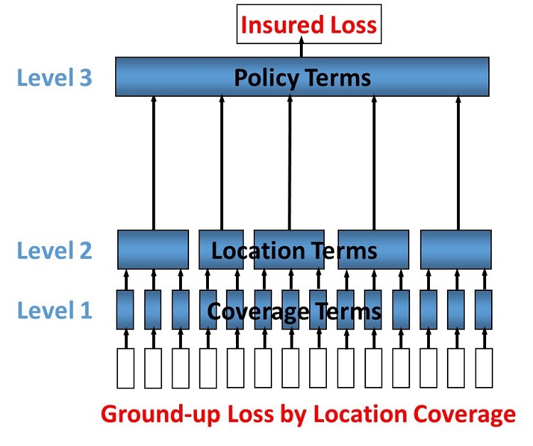
Groups are defined within levels and they represent aggregations of losses on which to perform the financial calculations. The grouping fields are called from_agg_id and to_agg_id which represent a grouping of losses at the previous level and the present level of the hierarchy, respectively.
Each level calculation applies to the to_agg_id groupings in the heirarchy. There is no calculation applied to the from_agg_id groupings at level 1 - these ids directly correspond to the ids in the loss input.
Figure 2. Example level 2 grouping

Loss values
The initial input is the ground-up loss (GUL) table, generally coming from the main Oasis calculation of ground-up losses. Here is an example, for a two events and 1 sample (idx=1):
event_id |
item_id |
sidx |
loss |
|---|---|---|---|
1 |
1 |
1 |
100,000 |
1 |
2 |
1 |
10,000 |
1 |
3 |
1 |
25,000 |
1 |
4 |
1 |
400 |
2 |
1 |
1 |
90,000 |
2 |
2 |
1 |
15,000 |
2 |
3 |
1 |
3,000 |
2 |
4 |
1 |
500 |
The values represent a single ground-up loss sample for items belonging to an account. We use “programme” rather than “account” as it is more general characteristic of a client’s exposure protection needs and allows a client to have multiple programmes active for a given period. The linkage between account and programme can be provided by a user defined prog dictionary, for example:
prog_id |
account_id |
prog_name |
|---|---|---|
1 |
1 |
ABC Insurance Co. 2016 renewal |
Items 1-4 represent Structure, Other Structure, Contents and Time Element coverage ground up losses for a single property, respectively, and this example is a simple residential policy with combined property coverage terms. For this policy type, the Structure, Other Structure and Contents losses are aggregated, and a deductible and limit is applied to the total. A separate set of terms, again a simple deductible and limit, is applied to the “Time Element” coverage which, for residential policies, generally means costs for temporary accommodation. The total insured loss is the sum of the output from the combined property terms and the time element terms.
Programme
The actual items falling into the programme are specified in the programme table together with the aggregation groupings that go into a given level calculation:
from_agg_id |
level_id |
to_agg_id |
|---|---|---|
1 |
1 |
1 |
2 |
1 |
1 |
3 |
1 |
1 |
4 |
1 |
2 |
1 |
2 |
1 |
2 |
2 |
1 |
Note that from_agg_id for level_id =1 is equal to the item_id in the input loss table (but in theory
from_agg_id could represent a higher level of grouping, if required).
In level 1, items 1, 2 and 3 all have to_agg_id =1 so losses will be summed together before applying the combined
deductible and limit, but item 4 (time element) will be treated separately (not aggregated) as it has to_agg_id
= 2. For level 2 we have all 4 items losses (now represented by two groups from_agg_id =1 and 2 from the previous
level) aggregated together as they have the same to_agg_id = 1.
Profile
Next we have the profile description table, which list the profiles representing general policy types. Our example is represented by two general profiles which specify the input fields and mathematical operations to perform. In this example, the profile for the combined coverages and time is the same (albeit with different values) and requires a limit, a deductible, and an associated calculation rule, whereas the profile for the policy requires a limit, attachment, and share, and an associated calculation rule.
Profile description |
calcrule_id |
|---|---|
deductible and limit |
1 |
deductible and/or attachment, limit and share |
2 |
There is a “profile value” table for each profile containing the applicable policy terms, each identified by a
policytc_id. The table below shows the list of policy terms for calcrule_id 1:
policytc_id |
deductible1 |
limit1 |
|---|---|---|
1 |
1,000 |
1,000,000 |
2 |
2,000 |
18,000 |
And next, for calcrule_id 2, the values for the overall policy attachment, limit and share:
policytc_id |
deductible1 |
attachment1 |
limit1 |
share1 |
|---|---|---|---|---|
3 |
0 |
1,000 |
1,000,000 |
0.1 |
In practice, all profile values are stored in a single flattened format which contains all supported profile fields (see fm profile here), but conceptually they belong in separate profile value tables.
The flattened file is:
fm_profile
policytc_id |
calcrule_id |
deductible1 |
deductible2 |
deductible3 |
attachment1 |
limit1 |
share1 |
share2 |
share3 |
|---|---|---|---|---|---|---|---|---|---|
1 |
1 |
1,000 |
0 |
0 |
0 |
1,000,000 |
0 |
0 |
0 |
1 |
1 |
2,000 |
0 |
0 |
0 |
18,000 |
0 |
0 |
0 |
1 |
2 |
0 |
0 |
0 |
1,000 |
1,000,000 |
0.1 |
0 |
0 |
For any given profile we have one standard rule calcrule_id, being the mathematical function used to calculate
the losses from the given profile’s fields. More information about the functions can be found
here.
Policytc
The policytc table specifies the (re)insurance contracts (this is a combination of agg_id and layer_id)
and the separate terms and conditions which will be applied to each layer_id/agg_id for a given level. In our
example, we have a limit and deductible with the same value applicable to the combination of the first three items, a
limit and deductible for the fourth item (time) in level 1, and then a limit, attachment, and share applicable at
level 2 covering all items. We’d represent this in terms of the distinct agg_ids as follows:
layer_id |
level_id |
agg_id |
policytc_id |
|---|---|---|---|
1 |
1 |
1 |
1 |
1 |
1 |
2 |
2 |
1 |
2 |
1 |
3 |
In words, the data in the table mean:
At Level 1:
Apply
policytc_id(terms and conditions) 1 to (the sum of losses represented by)agg_id1Apply
policytc_id2 to agg_id 2
Then at level 2:
Apply
policytc_id3 toagg_id1
Levels are processed in ascending order and the calculated losses from a previous level are summed according to the groupings defined in the programme table which become the input losses to the next level.
Layers
Layers can be used to model multiple sets of terms and conditions applied to the same losses, such as excess policies.
For the lower level calculations and in the general case where there is a single contract, layer_id should be set
to 1. For a given level_id and agg_id, multiple layers can be defined by setting layer_id =1,2,3 etc, and
assigning a different calculation policytc_id to each.
Figure 3. Example of multiple layers
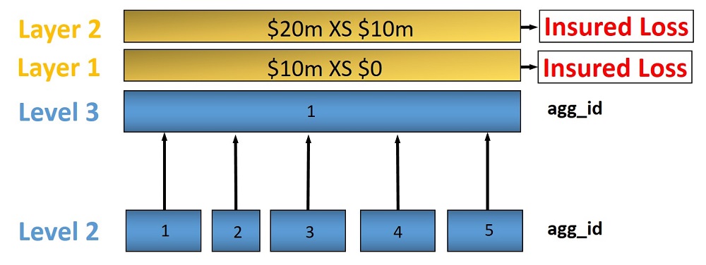
For this example at level 3, the policytc data might look as follows:
layer_id |
level_id |
agg_id |
policytc_id |
|---|---|---|---|
1 |
3 |
1 |
22 |
2 |
3 |
1 |
23 |
Output and back-allocation
Losses are output by event, output_id and sample. The table looks like this:
event_id |
output_id |
sidx |
loss |
|---|---|---|---|
1 |
1 |
1 |
455.24 |
2 |
1 |
1 |
345.6 |
The output_id is specified by the user in the xref table, and is a unique combination of agg_id and layer_id.
For instance:
output_id |
agg_id |
layer_id |
|---|---|---|
1 |
1 |
1 |
2 |
1 |
2 |
The output_id must be specified consistently with the back-allocation rule. Losses can either output at the
contract level or back-allocated to the lowest level, which is item_id, using one of three command line options.
There are three meaningful values here – don’t allocate (0) used typically for all levels where a breakdown of losses
is not required in output, allocate back to items (1) in proportion to the input (ground up) losses, or allocate back
to items (2) in proportion to the losses from the prior level calculation.
$ fmcalc -a0 # Losses are output at the contract level and not back-allocated
$ fmcalc -a1 # Losses are back-allocated to items on the basis of the input losses (e.g. ground up loss)
$ fmcalc -a2 # Losses are back-allocated to items on the basis of the prior level losses
The rules for specifying the output_ids in the xref table are as follows:
Rule 1: there is an
output_idfor everyagg_idandlayer_idof the final level in the policytc tableRule 2: there is an
output_idfor everyfrom_agg_idof the first level in the programme table, and for everylayer_idin the final level of the policytc table
To make sense of this, if there is more than one output at the contract level, then each one must be back-allocated
to all of the items, with each individual loss represented by a unique output_id.
To avoid unnecessary computation, it is recommended not to back-allocate unless losses are required to be reported at
a more detailed level than the contract level (site or zip code, for example). In this case, losses are re-aggregated
up from item level (represented by output_id in fmcalc output) in summarycalc, using the fmsummaryxref
table.
Reinsurance
The first run of fmcalc is designed to calculate the primary or direct insurance losses from the ground up losses of an exposure portfolio. fmcalc has been designed to be recursive, so that the ‘gross’ losses from the first run can be streamed back in to second and subsequent runs of fmcalc, each time with a different set of input files representing reinsurance contracts, and can output either the reinsurance gross loss, or net loss. There are two modes of output:
gross meaning the loss to the policies or reinsurance contracts, and
net being the difference between the input loss and the policy/contract losses
net loss is output when the command line parameter -n is used, otherwise output loss is gross by default.
Supported reinsurance types
The types of reinsurance supported by the Financial Module are:
Facultative proportional or excess
Quota share with event limit
Surplus share with event limit
Per risk with event limit
Catastrophe excess of loss occurrence only
Required files
Second and subsequent runs of fmcalc require the same four fm files fm_programme, fm_policytc, fm_profile,
and fm_xref.
This time, the hierarchy specified in fm_programme must be consistent with the range of output_ids from the
incoming stream of losses, as specified in the fm_xref file from the previous iteration. Specifically, this means
the range of values in from_agg_id at level 1 must match the range of values in output_id.
For example:
fm_xref (iteration 1)
output_id |
agg_id |
layer_id |
|---|---|---|
1 |
1 |
1 |
2 |
1 |
2 |
fm_programme (iteration 2)
from_agg_id |
level_id |
to_agg_id |
|---|---|---|
1 |
1 |
1 |
2 |
1 |
2 |
1 |
2 |
1 |
2 |
2 |
1 |
The abstraction of from_agg_id at level 1 from item_id means that losses needn’t be back-allocated to
item_id after every iteration of fmcalc. In fact, performance will be improved when back-allocation is minimised.
Inuring priority
The Financial Module can support unlimited inuring priority levels for reinsurance. Each set of contracts with equal inuring priority would be calculated in one iteration. The net losses from the first inuring priority are streamed into the second inuring priority calculation, and so on.
Where there are multiple contracts with equal inuring priority, these are implemented as layers with a single iteration.
The net calculation for iterations with multiple layers is:
net loss = max(0, input loss - layer1 loss - layer2 loss - … - layer n loss)
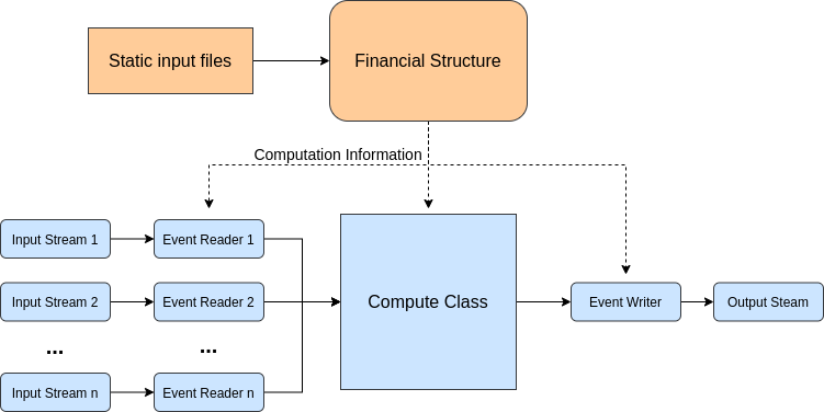
Financial module architecture design
Manager is the high level entry point to run an Financial Module computation. It orchestrates the different modules together in order to process the incoming events. Each event is read one at a time from available input streams. We then compute the result and write it to the output stream.
The basic idea of the architecture of the Financial Module is that, in each event, we only compute nodes that need it. When an event is read, the node_id corresponding to each item is added to a “computes” queue. During the bottom up part, where losses are aggregated to higher levels, the loss of a nodeis computed and then its parent node is added in the queue. The node is also added to the list of active children for the parent node. This way the parent node only aggregate the loss of active children.
During back-allocation, the process is repeated, but this time its the parent node that adds its children to the ‘compute’ queue.
Overall the fm computation is done in two steps:
1. Creation of the shared static financial structure files. ex: fmpy --create-financial-structure-files -a 2
2. Event computation ex: fmpy -i stream_in -o stream_out -a 2
Financial Structure
The purpose of this module is to parse the static input financial structure and consolidate the information into simple objects ready to be use by the compute function. The idea is to factorise all the computation and logic that can be done at this step and prepare everything possible to have a generic way to handle the computation for each item.
The object created during the financial structure step are all numpy ndarrays. This presents many advantages.
numpy provides an easy way to have them stored.
They can be loaded as a shared memory objects for all the compute processes, which greatly reduces memory usage.
They are very fast and compact.
In particular, those are preferred to the numba dictionaries and lists, even when it would be simpler to use because they are much faster at the moment (early 2021). This means that all the references from an objet to other objects need to be done via a pointer like logic. For example, the node ids of the parents of a node are referenced in node_array with a length (parent_len) and the index of the first parent id in node_parent_array.
Inputs
The necessary static inputs for the Financial Module are expected to be in the same folder with the extention
‘.bin’ for binaries and ‘.cvs’ for text files:
fm_programme: the basic hierarchy of nodes organised by level and aggregation idfm_policytc: the policy id to apply to each node and layer described in the programmefm_profileorfm_profile_step: the profile (detailed values) of each policy idfm_xref: the mapping between result items and the output ID
Additionally if %tiv policies are present, those two extra files will be needed:
items: link between
item_idandcoverage_idcoverage: link between
coverage_idandTIV
In productions, inputs are read directly using numpy.fromfile, with named dtype specific to each file name. This allows one to access each value in a row like a dictionary and also provide a compatible interface for the two profile options (step or non step policy). We make a realistic assumption that the input and output data will fit in memory.
Outputs
The transform static information needed to build and execute the computation for each event:
compute_info: Contains the general information on the financial structure such as the allocation rule, the number of levels and whether there is stepped policy. It also contains the length of all the other ndarrays.
nodes_array: All the static information about a node, such as
level_id,agg_id, number of layers, and number of policies. Referenced to its parents, children, profiles and different loss array.node_parents_array: Contains the index of parent node in
node_array.node_profiles_array: Contains the index of the node profile in
fm_profile.output_array: Contains the
item_idof the output losses of each layer of a node (generated from xref).fm_profile: Contains the final version of all the policies in the original
fm_profile(for example, we compute the real tiv in order replace all %tiv policy values).
Computation
The computation of the loss itself can only be done after the financial structure creation step.
The manager module will then load this shared structure and then create all the dynamic arrays:
losses and loss_indexes: arrays to reference and store all losses.
extras and extra_indexes: arrays to reference and store the extra values such as
deductible,under_limit, andover_limit.children: array of active children for each parant node.
computes: contains the index of all the nodes to compute.
One thing to note with this architecture is that a node doesn’t really ‘own’ its different losses. It only has a reference to it via loss_indexes. This is very important as it allows us to share the array between nodes if they happen to be the same. As we only copy the reference, this drastically reduces the amount of data copied in several cases.
When a parent node has only one active child, then the aggregation of losses is not needed. The parent node
sum_losswill simply point to its childrenil_loss.When a node has a pass through profile (id 100), it’s
il_losswill point to itssum_loss.During the back allocation, if a parent has only one child, the
ba_lossof the child will simply point to theba_lossof the parent.
Once those structures are created, the manager will orchestrate the processes event by event:
1. An event is read - all the items of the event are placed in the compute queue.
2. An incremental pointer to computes compute_i tracks which nodes need to be computed. The computation starts with the bottom up step. For each node, we aggregate the sub loss, apply the profile, and put the parent node in the queue. If the value it points to is 0, we are at the end of the level and can go to the next one. Then, depending on rule, we continue the same logic for the back allocation, only this time it goes from parent to children.
3. The stream writer reads the last level of ‘computes’ and writes each active item and its loss to the output stream.
Policies
The policy module contains all the functions associated to the supported policy. They all take the same numpy array as input and acts directly on them (inplace).
Signature: calcrule_i(policy, loss_out, loss_in, deductible, over_limit, under_limit) loss is present in two arrays because, in some cases, we want to keep the sum value before the calc rule is applied (if this is not the case, the arrays are the same object).
Stream
The stream module is responsible for the parsing and writing of the gul and fm streams. The stream reader is able to read from multiple streams using the selector module of python.