Modelling methodology
On this page
What is a catastrophe model
Catastrophe models are used extensively in the (re)insurance industry to estimate expected losses from natural disasters. Catastrophe models output loss exceedance curves (LECs), i.e. a probability distribution of losses that will be sustained by an insurance company in any given year, together with an annual average loss (AAL) and standard deviation. Given the paucity in historical losses for extreme events from which to build actuarial based models, catastrophe models take a bottom-up approach from scientific first principles to estimate the risk.
The anatomy of a typical catastrophe model is shown below:
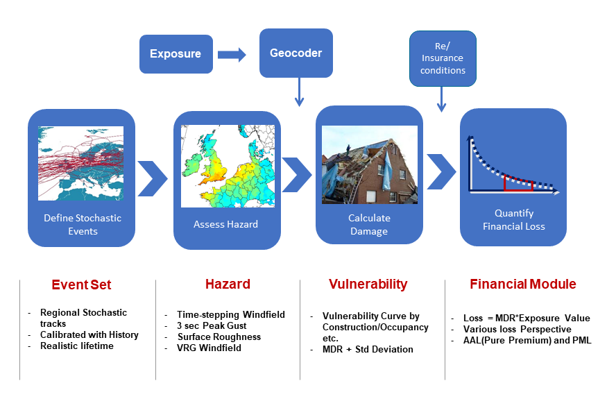
Anatomy of a catastrophe model
The first task is to generate an event set representative of all possible events that may occur, along with their intensity and probability across a long-enough time period to encapsulate a comprehensive distribution of even the most extreme events. A 10,000 year simulation is often used. The goal is not to recreate the last 10,000 years of history, but to simulate 10,000 years of activity equivalent to current conditions. Each event has a probability of occurrence within the simulated time period. Models often employ a “boiling down” process to optimise the run-times of their models by combining very similar events together, including their probability of occurrence. This maintains the representativeness of the ultimate event set to be consistent with the original event set in terms of losses and the geographical distribution of loss, but is faster for the user to run.
For each event a hazard footprint will be generated, which calculates an appropriate hazard metric which correlates to damage at each point in a grid across the entire area effected by an event. For example, this is may be the maximum 3-second peak gust experienced at every location by a windstorm during the course of that windstorm. Time-stepping models are used which simulate the storm and its windfield say every 15 minutes throughout the entire lifecycle of the storm, which may be many hours in duration. Topography, surface roughness, soil and geological information must all be taken into account, as the model is representing the hazard at the surface of the ground. The maximum peak-gust windspeed experienced is stored as the “hazard footprint” provided by a catastrophe model.
Vulnerability curves link the hazard metric (e.g. 3-second peak gust or flood depth) to a Mean Damage Ratio (MDR), the proportion of the total value (e.g. in terms of replacement cost) that would be a loss for the asset being analysed. In reality, properties exhibit a high amount of variability in their damage to the same hazard due to many unknown and un-modellable factors, even when located very close to each other. This is accounted for in an uncertainty distribution around the mean damage ratio at each hazard point, also known as “secondary uncertainty”. Models will often define different vulnerability zones across a region to account for different building practices or building codes.
A financial module calculates losses after taking into account the impact of insurance company policy terms and conditions to provide the net loss that the (re)insurance entity will ultimately be responsible for. The (re)insurance company enters a list of all the policies it has underwritten with information about the location and risk characteristics, such as occupancy type, age, construction material, building height, and replacement cost of the building, as well as policy terms & conditions. The catastrophe model will then run the entire event set across the portfolio, and calculate a loss from every event in the model to every policy. This produces an event loss table. These event losses are then ordered in terms of magnitude from largest to smallest to generate the Loss Exceedance Curve for the number of years the model simulates.
Catastrophe models typically cover single peril-region combinations, e.g. Europe windstorm, Japanese earthquake. Whilst average annual losses from each peril-region combination analysis can be added together, loss exceedance curves cannot and must be recalculated after different peril-region analyses have been grouped together. This is because of the diversifying nature of writing risk in different, uncorrelated regions, or conversely because two portfolios have a very similar risk profile and are correlated, and therefore the combined return-period risk may be more or less than the sum of the two.
Catastrophe model loss results output varies considerably between different developers, due to differences in data, assumptions, modelling techniques etc. Users can validate models against observational data, losses, and claims data if they have them at a detailed level. This takes significant expertise, for example if comparing model windspeeds against observed windspeeds, care must be taken to account for the fact that windspeed observations are usually recorded at a standard height above ground level. However, the catastrophe model is simulating surface windspeeds, and incorporating the effect of surface roughness and upwind obstacles such as trees and buildings in this calculation. Data only exists at lower return periods of course, therefore qualitative expert judgement will be used to evaluate a model appropriateness and fit-for-purpose.
Simulation methodology
The Oasis kernel provides a robust loss simulation engine for catastrophe modelling.
Insurance practitioners are used to dealing with losses arising from events. Policy terms are applied to the losses individually and then aggregated and further conditions or reinsurances applied.
Oasis takes the same approach in the modelling of losses, which is to generate individual losses from the damage probability distributions. The way to achieve this is random sampling called “Monte-Carlo” sampling from the use of random numbers, as if from a roulette wheel, to solve equations that are otherwise intractable.
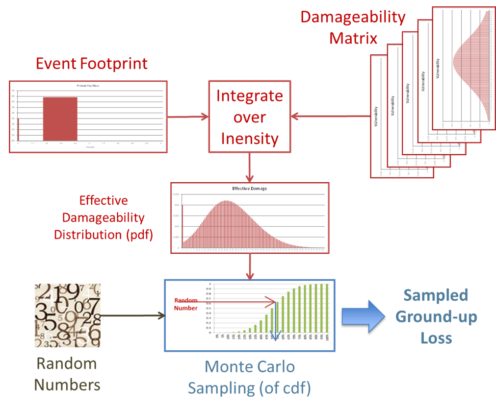
Modelled and empirical intensities and damage responses can show significant uncertainty. Sometimes this uncertainty is multi-modal, meaning that there can be different peaks of behaviour rather than just a single central behaviour. Moreover, the definition of the source insured interest characteristics, such as location or occupancy or construction, can be imprecise. The associated values for event intensities and consequential damages can therefore be varied and their uncertainty can be represented in general as probability distributions rather than point values. The design of Oasis therefore makes no assumptions about the probability distributions and instead treats all probability distributions as probability masses in discrete bins. This includes closed interval point bins such as the values [0,0] for no damage and [1,1] for total damage.
The simulation approach taken by the Oasis calculation kernel computes a single cumulative distribution function (CDF) for the damage by “convolving” the binned intensity distribution with the vulnerability matrices. The convolution applies the ‘law of total probability’ to evaluate the overall probability of each damage outcome, by summing the probability of all levels of intensity multiplied by the conditional probability of the damage outcome in each case.
Sampling of the cumulative distribution function is then performed. Random numbers between 0 and 1 are drawn, and used to sample a relative damage ratio from the effective damage CDF. Linear interpolation of the cumulative probability thresholds of the bin in which the random number falls is used to calculate the damage ratio for each sample.
Finally, a ground up loss sample is calculated by multiplying the damage ratio with the Total Insured Value ‘TIV’.